This description of the backpropagation algorithm is derived from D. E. Rumelhart, G. E. Hinton, and R. J. Williams: Parallel Distributed Processing (PDP), Vol. 1 pages 318-362, MIT Press 1986. This was the first time that the gradient descent optimization algorithm was described in the context of machine learning.

Nowadays backpropagation is usually described as a probabilistic approach to estimate unknown distributions by maximizing a likelihood estimation. See for example Goodfellow, Ian, Bengio, Yoshua, and Courville, Aaron. Deep Learning, MIT Press, 2016. Website: www.deeplearningbook.org

Architecture

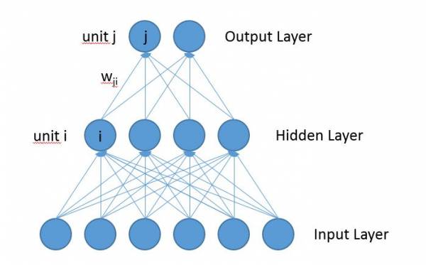
A Multi-Layer Perceptron (MLP) consists of several layers: one input layer, zero, one or several hidden layers, and one output layer. Every layer has one or several units. The activation of the units flows from the input layer through the hidden layers to the output layer. Every unit in one layer is connected to all units in the next upper layer. All connections are weighted with weights \(w\). A connection from unit \(i\) to unit \(j\) is weighted with the weight \(w_{ji}\). The following picture shows the architecture of an MLP:

Forward Pass

Input units are set to a specific value as the input.
All other units \(j\) compute their activation value \(o_j\) with the activation function \(f\):

\begin{equation}
o_j = f(net_j)
\end{equation}

\(net_j\) is the network input of unit \(j\), which is the weighted sum of the activations \(o_i\) of all units \(i\) which are connected to unit \(j\). \(w_{ji}\) is the weight from unit \(i\) to unit \(j\):

\begin{equation}
net_j = \sum_i w_{ji} o_i
\end{equation}

\begin{equation}
o_j = f(\sum_i w_{ji} o_i)
\end{equation}

All units \(j\) except the input units can have a bias value \(b_j\) as an additional parameter, which is also included in the sum in equation (2). However, the bias value can be viewed as an additional weight \(w_{jb}\) to a bias unit \(b\) with the constant output value \(o_b = 1\). Equation (2) is still valid.

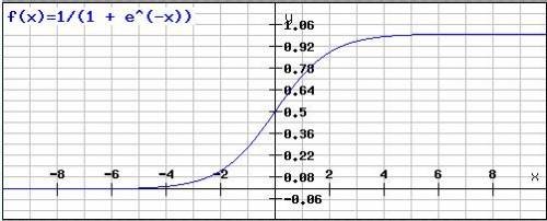
To perform a nonlinear classification, the activation function \(f\) has to be nonlinear, like a threshold function for example. On the other side, the gradient descent learning algorithm requires that the activation function is derivable. A popular function for \(f\) which fulfills these requirements is the logistic sigmoid function:

\begin{equation}
f(net_j) = \frac{1}{1 + e^{-net_j}}
\end{equation}

The logistic sigmoid function is defined for all values \(-\infty \leq x \leq \infty\) with an output \(0 \leq f(x) \leq 1\). The following picture shows the function graph of the logistic sigmoid function:

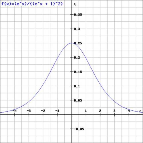
The derivation of the logistic sigmoid function (4) is:

\begin{equation}
f'(x) = \frac{e^{x}}{(e^{x} + 1)^{2}}
\end{equation}

The following picture shows the function graph of the derivation of the logistics sigmoid function:

After setting the input unit to a specific input pattern, the activation of all units in the different layers are calculated layer by layer up to the output layer by the formulas described above. The activation of the units of the output layers is the output of the network based on the input activations.

Backward Pass

In the backward pass, the weights of the network are adjusted in order to minimize the error of the network with respect to the desired input-output functionality. We call this the learning algorithm.

If the input layer consists of \(n\) units and the output layer consists of \(m\) units, the backpropagation network computes a mapping from an \(n\)-dimensional vector space \(I^n\) to a \(m\)-dimensional vector space \(O^m\):

\begin{equation}
I^n \rightarrow O^m
\end{equation}

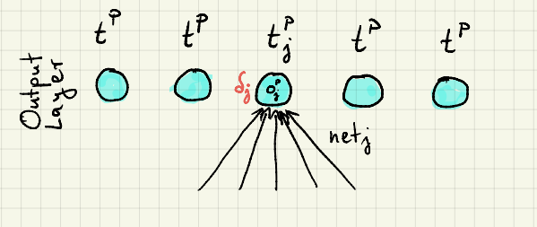
In the training phase, the desired behavior is specified to the network by input-output pairs \((i^p, t^p)_{p = 1..P}\) consisting of \(P\) pairs of an input vector \(i^p\) and a target vector \(t^p\). The set of these pairs is called the training set.

By presenting the input vector \(i^p\) to the network, it computes the output vector \(o^p\) with the forward pass. The error between the actual output vector \(o^p\) and the desired target vector \(t^p\) can be computed by the squared \(L^2\) norm or the Squared Euclidean Distance:

\begin{equation}
E^P = \sum_i (o_i^p – t_i^p)^2
\end{equation}

The overall error over the entire training set \(1..P\) can be expressed by the mean error:

\begin{equation}
E = \frac{1}{P} \sum_{p=1}^{P} E^p
\end{equation}

One way to search for the desired weights \(w_{ji}\) which minimizes the error \(E\) is the gradient descent technique. For every weight \(w_{ji}\) from unit \(i\) to unit \(j\) the derivation of the error function \(E\) (formula 8) with respect to the weight \(w_{ji}\) is calculated and the weight is changed in the opposite direction of the gradient:

\begin{equation}
\Delta w_{ji} =\ – \eta \frac{\partial E}{\partial w_{ji}}
=\ – \eta \frac{1}{P}\sum_{p=1}^P \frac{\partial E^p}{\partial w_{ji}}
\end{equation}

\(\eta\) specifies the amount of the weights change and is called the learning rate.

We can calculate the gradient by using the chain rule:

\begin{equation}
\frac{\partial E^p}{\partial w_{ji}} = \frac{\partial E^p}
{\partial net_j^p}\frac{\partial net_j^p}{\partial w_{ji}}
\end{equation}

\begin{equation}
\frac{\partial net_j^p}{\partial w_{ji}} = \frac{\partial \sum_k w_{jk} o_k^p}{\partial w_{ji}}
= \frac{\partial w_{ji} o_i^p}{\partial w_{ji}}= o_i^p
\end{equation}

By defining:

\begin{equation}
\delta_j^p = \frac{\partial E^p}{\partial net_j^p}
\end{equation}

We can write:

\begin{equation}
\frac{\partial E^p}{\partial w_{ji}} = \delta_j^p o_i^p
\end{equation}

To compute \(\delta_j^p\) we have to distinguish two cases:

1. case: Unit \(j\) belongs to the output layer
2. case: Unit \(j\) belongs to a hidden layer

1. case: Unit \(j\) belongs to the output layer:

\begin{align}
\delta_j^p &= \frac{\partial E^p}{\partial net_j^p} \\
&= \frac{\partial \sum_i(o_i^p – t_i^p)^2}{\partial net_j^p} \\
&= \frac{\partial \sum_i(f(net_i^p) – t_i^p)^2}{\partial net_j^p} \\
&= \frac{\partial (f(net_j^p) – t_j^p)^2}{\partial net_j^p} \\
&= 2 (f(net_j^p) – t_j^p) f'(net_j^p) \\
&= 2 (o_j^p – t_j^p) f'(net_j^p)
\end{align}

2. case: Unit \(j\) belongs to a hidden layer. Now unit \(j\) does not contribute directly to the error but through the units in the descendant layers:

\begin{align}
\delta_j^p &= \frac{\partial E^p}{\partial net_j^p}
= \frac{\partial E^p}{\partial o_j^p} \frac{\partial o_j^p}{\partial net_j^p}
\end{align}

\begin{equation}
\frac{\partial o_j^p}{\partial net_j^p} = \frac{\partial f(net_j^p)}{\partial net_j^p} = f'(net_j^p)
\end{equation}

\begin{equation}
\delta_j^p = \frac{\partial E^p}{\partial o_j^p} f'(net_j^p)
\end{equation}

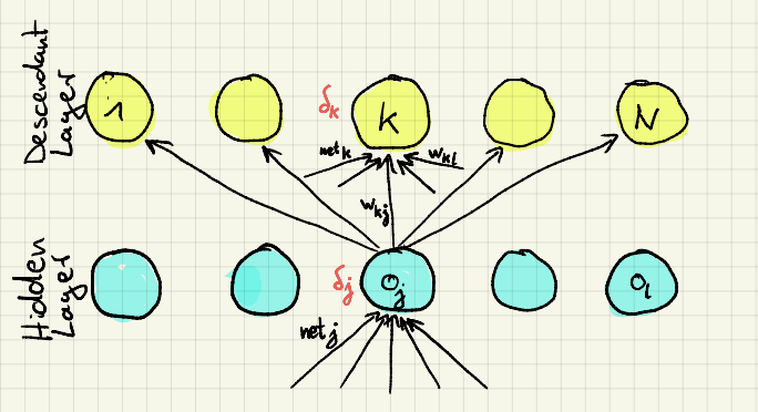
To compute the dependence of the error \(E^p\) from the output of the hidden unit \(j\), we look at how the output of unit \(j\) influences the error in the output layer. We see that the output of unit \(j\) influences only the net input of all units \(1..N\) in the successive layer directly. The error at the output layer depends on the net inputs of these units.

\begin{align}
\frac{\partial E^p}{\partial o_j^p} &= \sum_{k=1}^{N} \frac{\partial E^p}{\partial net_k^p}
\frac{\partial net_k^p}{\partial o_j^p} \\
&= \sum_{k=1}^{N} \frac{\partial E^p}{\partial net_k^p}
\frac{\partial \sum_l w_{kl} o_l^p}{\partial o_j^p} \\
&= \sum_{k=1}^{N} \frac{\partial E^p}{\partial net_k^p}
\frac{\partial w_{kj} o_j^p}{\partial o_j^p} \\
&= \sum_{k=1}^{N} \frac{\partial E^p}{\partial net_k^p} w_{kj} \\
&= \sum_{k=1}^{N} \delta_k^p w_{kj}
\end{align}

\begin{equation}
\delta_j^p = (\sum_k \delta_k^p w_{kj}) f'(net_j^p)
\end{equation}

So \(\delta_j\) of a unit \(j\) in a hidden layer is dependent on all \(\delta_k^p\) of the units \(k\) in the descendent layer which are connected to unit \(j\) via the weight \(w_{kj}\). This way the deltas are “backpropagated” from the upper layers to the lower layers.

Learning Algorithm

For every input-output pair \((i^p, o^p)_{p = 1..N}\) of the training set, the unit activations have to be computed by the forward pass.

Then the deltas of all units in the output layer for the input-output pair \(p\) have to be computed by equation (19):

\begin{equation}
\delta_j^p = 2 (o_j^p – t_j^p) f'(net_j^p)
\end{equation}

Now the deltas can be computed by the next lower layer by backpropagation the deltas from the output layer to the next lower layer with equation (28):

\begin{equation}
\delta_j^p = (\sum_k \delta_k^p w_{kj}) f'(net_j^p)
\end{equation}

This procedure is repeated down to the lowest hidden layer (the input layer has no weights and no deltas need to be computed).

After the deltas are computed for all units in all hidden layers for all input-output pairs \(p\), the weights can be changed:

\begin{equation}
\Delta w_{ji} = – \eta \frac{1}{P}\sum_{p=1}^P \delta_j^p o_i^p
\end{equation}

For one weight change, the whole training set has to be processed. Especially for larger training sets, this is impractical. Therefore today usually Stochastic Gradient Descent (SGD) is used instead. For SGD, a randomly selected subset of the training set with 1 to several hundred training patterns is used to calculate one weight change.